Hi!

This notebook aims at providing details about our segmentation algorithm, as it was entirely developped for our context of segmenting music with NTD, and is in that sense "non-standard".

We considered important to provide these details here as it wasn't the main priority in the article, limited in space.

NB: this notebook contains images and gifs, which don't appear in the gitlab presentation page, or if you don't download the imgs folder. Hence, you should download either the HTML or the jupyter notebook, along with the imgs folder.

Our algorithm in a nutshell¶

We developed a dynamic programming algorithm adapted for segmenting sparse autosimilarity matrices.

The main idea is that, the darker is the zone we analyze, the more similar it is, and hence the more probable this zone belongs to a same segment.

Below, we illustrated the main principle of our algorithm on a toy autosimilarity matrix, which is framing all dark blocks.

Given the autosimilarity matrix of the factor $Q$ of NTD, we apply kernels of different sizes around its diagonal, and search for the sequence of segments which will maximize a certain cost, defined, for each segment, as the convolution between the kernel and the autosimilarity matrix, cropped.

Concretely, the convolution cost for a segment ($b_1$, $b_2$) is the sum of the term-to-term product of the kernel and the autosimilarity of this segment, centered on the diagonal and cropped to the boundaries of the segment (i.e. the autosimilarity restricted to the indexes $(i,j) \in [b_1, b_2]^2$). The kernel and the autosimilarity must be of the same size.

As segments could be of different sizes, and as our kernels and (cropped) autosimilarities are squared matrices, the sum involves (size of the segment)$^2$ elements. This isn't desirable as large blocks will be favoured by this squared term. In that sense, we then normalize this sum by the size of the segment.

Mathematically, this means: $c_{b_1,b_2} = \frac{1}{b_2 - b_1 + 1}\sum_{i,j = 0}^{n - 1}k_{ij} a_{i + b_1, j + b_1}$ by denoting $k_{ij}$ the elements of the kernel and $a_{i,j}$ the elements of the autosimilarity matrix.

Starting from this cost for a segment, we aim at finding the sequence of segments maximizing the sum of local convolution costs.

To this end, we use a dynamic programming algortihm (inspired from [1]) which tries to maximize the global sum of all costs of a sequence of segments:

We iterate over all bars of the music, in temporal order, considering them as segment ends. Let's denote $b_e$ one of these bars.
We then iterate over all bars which could start a segment ending at $b_e$ (here, all previous bars could start the segment, as long as the segment is shorter than 36 bars). Let $b_s$ be one of these potential starts, and $S_{starts}$ the set of all these bars.
We compute the convolution cost associated with this segment [$b_s$, $b_e$], which we denote $c_{s,e}$.
Having iterated over all previous bars, we know the optimal segmentation between the start of the music and the bar $b_s$, considering $b_s$ as the end of a segment. We can make this assumption as segmenting the music before $b_s$ is a different problem than segmenting after $b_s$ if we fix $b_s$ as an end of segment. Hence, we have the cost $c_{0,s}$, cost of the optimal segmentation ending at $b_s$, and so we define $c_{0,s,e} = c_{0,s} + c_{s,e}$.
Hence, iterating over the $b_s \in S_{starts}$, we compute a set of costs $\{c_{0,s,e}\}$. As a numerical and finite set, it admits a maximum for a bar $b_s^{opt} \in S_{starts}$, and we define $c_{0,e} = c_{0,s^{opt},e}$, and stores $b_s^{opt}$ as the best start for a segment ending at $b_e$. Hence, the optimal segmentation for ending a segment at bar $b_e$ is the segmentation happening before $b_s^{opt}$ and the segment [$b_s^{opt}$, $b_e$].

For example, in a scenario with one particular $b_e$ and only 3 bars in $S_{starts}$ (for simplification): $b_s, b_s^{'}$ and $b_s^{''}$: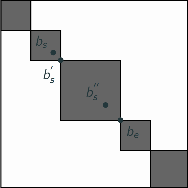

With these 3 possible segments are 3 respective costs for a segmentation ending at $b_e$:

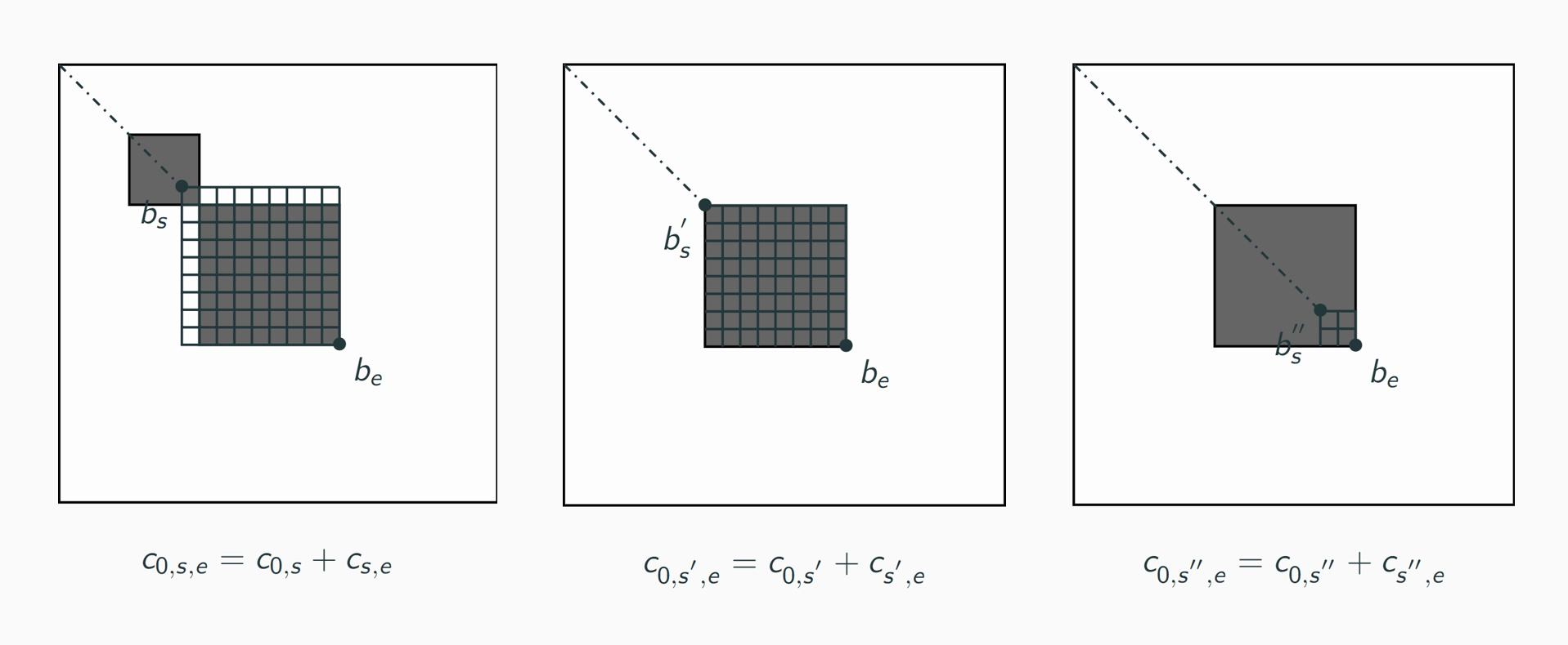
Finally, $c_{0,e} = max(c_{0,s,e}, c_{0,s^{'},e}, c_{0,s^{''},e}) = c_{0,s^{'},e}$, and, for $b_e$, $b_s^{opt} = b_s^{'}$.

At the last iteration (having parsed all bars of the music), we compute the optimal segmentation for ending at the last bar of the music, and find the optimal segment to end at the end of the song. We have found the optimal start $b_s^{opt}$ for the last bar of the song. Now, considering this start $b_s^{opt}$ as the end of the previous segment, we obtain the previous optimal segment, and etc. We then obtain the optimal segmentation by rolling back all optimal starts that we have computed.

This algorithm then returns the sequence of segments which maximizes the sum of all segment cost, among all possible segments in this song.

Details of the kernel¶

The idea we wanted to implement is to evaluate segments via the quantity of dark areas outside from the diagonal. Indeed, the diagonal will always be highly similar (as it represent the self-similarity of this bar, and it will even be equal to 1 as we normalize the autosimilarity barwise), and will dominate the other values of similarity.

In our idea, a dark block should indicate a zone of high similarity (as in the mock example shown in the first gif, where the algorithm frame all dark squares), and should then probably represent a structural segment.

Given this idea, several kernels can be imagined.

We imagined 3 of them, which we will present here. For tests and comparisons on real data of these kernels, report to the three associated notebooks (which starts by number 5).

Full kernel¶

The first we imagined is a "full kernel", where all values are equal to one (except on the diagonal).

It looks like: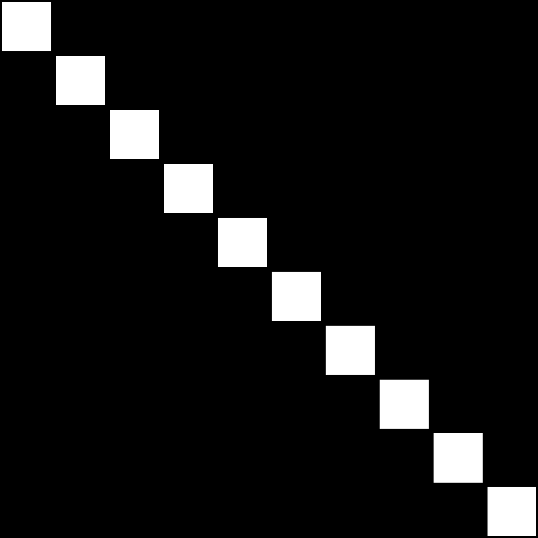

(or, in a matrix form: $\left[ \begin{matrix} 0 & 1 & 1 & 1& 1 & 1 & 1 & 1\\ 1 & 0 & 1 & 1& 1 & 1 & 1 & 1\\ 1 & 1 & 0 & 1& 1 & 1 & 1 & 1\\ 1 & 1 & 1 & 0 & 1 & 1 & 1 & 1\\ 1 & 1 & 1 & 1 & 0 & 1 & 1 & 1\\ 1 & 1 & 1 & 1 & 1 & 0 & 1 & 1\\ 1 & 1 & 1& 1 & 1 & 1 & 0 & 1\\ 1 & 1 & 1& 1 & 1 & 1 & 1 & 0\\ \end{matrix} \right]$ (of size 8 here)).

Mathematically, for a segment ($b_1, b_2$), the associated cost will be $c_{b_1,b_2} = \frac{1}{b_2 - b_1 + 1}\sum_{i,j = 0, i \ne j}^{n - 1} a_{i + b_1, j + b_1}$.

By construction, this kernel catches the similarity everywhere around the diagonal. As high similarity means higher values (and dark zones) in our autosimilarities, the higher this cost, the more similar is the zone we are studying.

In that sense, it should fulfil the need presented before in our simple example, which is framing dark squares.

In real world data though, autosimilarities are less simple than in our example.

For example, let's take the autosimilarity of Come Together that we present in our article: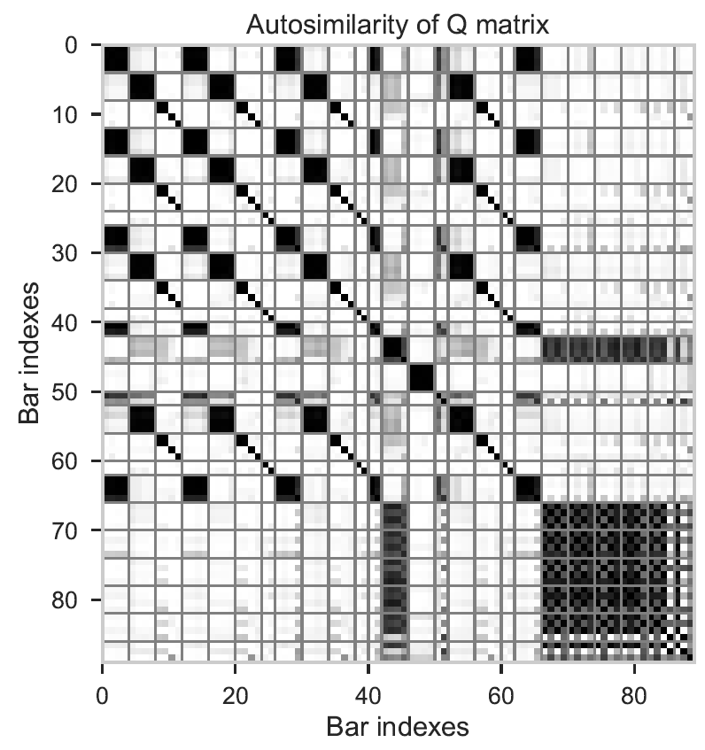

In this example, we notice a dark block at then end, which is annotated as 5 different segments: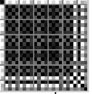

In such a similar zone, our kernel will favoure framing the entire block rather than segmenting it in 5 different segments, and it will surely result in 4 False Negatives.

Analogously, a structural block can be repeated, resulting in a highly similar block, but be labeled as two segments (and contain a frontier). This is represented in this example: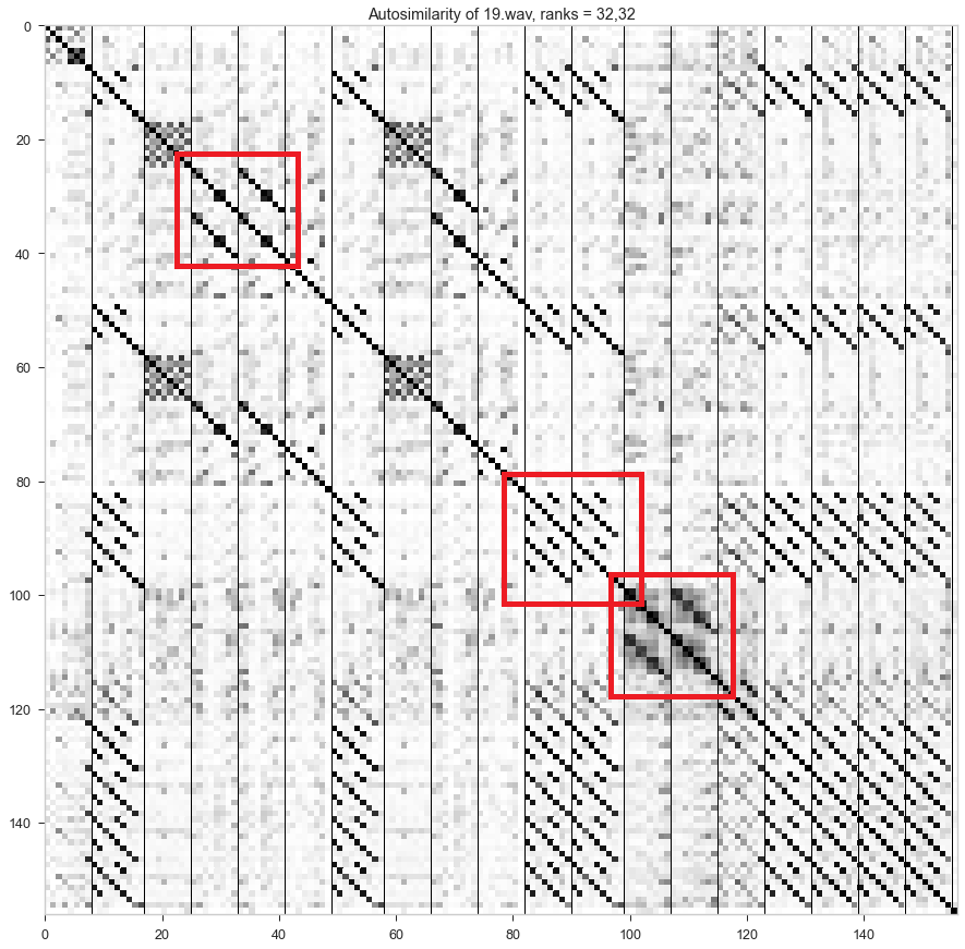

Above is shown the autosimilarity matrix of the song "19.wav" of RWC Pop when decomposed with ranks 32 for both $H$ and $Q$, in our algorithm.

In the 3 zones framed in red, we notice a highly similar zone, but containing a frontier that we'd like to find. Our full kernel would favoure segments lasting 16 bars at these 3 places, resulting in 3 False Negatives.

8 bands kernel¶

To solve this problem, we developed a second kernel, which focuses on local similarities in the 8 bars surrounding each bar of the diagonal (4 bars in the future, 4 bars in the past). Concretely, this kernel is a matrix where the only non-zero elements are the 8 closest bands parallel to the diagonal.

It looks like: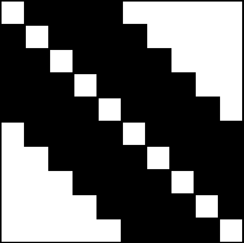

(or, in a matrix form: $\left[ \begin{matrix} 0 & 1 & 1 & 1& 1 & 0 & 0 & 0\\ 1 & 0 & 1 & 1& 1 & 1 & 0 & 0\\ 1 & 1 & 0 & 1& 1 & 1 & 1 & 0\\ 1 & 1 & 1 & 0 & 1 & 1 & 1 & 1\\ 1 & 1 & 1 & 1 & 0 & 1 & 1 & 1\\ 0 & 1 & 1 & 1 & 1 & 0 & 1 & 1\\ 0 & 0 & 1& 1 & 1 & 1 & 0 & 1\\ 0 & 0 & 0& 1 & 1 & 1 & 1 & 0\\ \end{matrix} \right]$ (of size 8 here)).

Mathematically, for a segment ($b_1, b_2$), the associated cost will be $c_{b_1,b_2} = \frac{1}{b_2 - b_1 + 1}\sum_{i,j = 0, 1 \leq |i - j| \leq 4}^{n - 1} a_{i + b_1, j + b_1}$.

With this kernel, we hoped to focus on local similarities, and to solve the segment-repetition problem.

Experiments at that time (not represented here, sorry!) tended to show that, indeed, our algorithm was more able to find frontiers in repeated blocks, but, in the same time, had more difficulties with larger segments with little local similarities.

Mixed kernel¶

In that sense, we developed a third kernel, which is a trade-off between local and "longer" term similarities.

Concretely, it is a sum of both previous kernels. It is composed of 0 in its diagonal, 2 in the 8 bands surrounding the diagonal, and 1 elsewhere.

It looks like: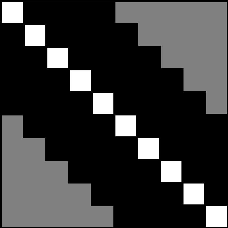

(or, in a matrix form: $\left[ \begin{matrix} 0 & 2 & 2 & 2& 2 & 1 & 1 & 1\\ 2 & 0 & 2 & 2 & 2& 2 & 1 & 1\\ 2&2 & 0 & 2 & 2 & 2& 2 & 1\\ 2&2&2 & 0 & 2 & 2 & 2& 2\\ 2 & 2 & 2& 2 & 0 & 2&2&2\\ 1 & 2 & 2 & 2& 2 & 0 & 2&2\\ 1 & 1 & 2 & 2 & 2& 2 & 0 & 2\\ 1 & 1 & 1& 2 & 2 & 2& 2 & 0\\ \end{matrix} \right]$ (of size 8 here)).

Mathematically, for a segment ($b_1, b_2$), the associated cost will be $c_{b_1,b_2} = \frac{1}{b_2 - b_1 + 1}(\sum_{i,j = 0, i \ne j}^{n - 1} a_{i + b_1, j + b_1} + \sum_{i,j = 0, 1 \leq |i - j| \leq 4}^{n - 1} a_{i + b_1, j + b_1})$.

It's called mixed kernel as it mixes both previous paradigms.

Future kernels¶

Finally, these three kernels are based on the hypothesis that structural blocks look like dark squares in the autosimilarity. In real-world data, this might not be the case, and the algorithm can fail. In that sense, future work could concern the design of new kernels, and even finding new segmentation algorithm (for example, segmenting the $Q$ matrix directly).

Penalty function¶

The study of the MIREX10 annotations in [1] shows that segments in this dataset are regular, and mostly centered around the size of 16 onbeats.

We replicated these results by studying the size in number of bars, more adapted to our context.

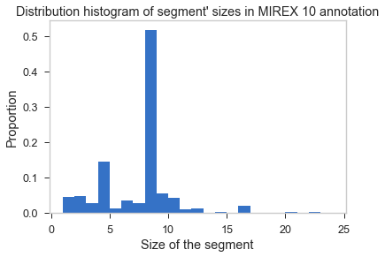
We see in this histogram that most of the segment (more than a half) last 8 bars, and that numerous other segments last 4 bars. The other values are less represented. Hence, it should be interesting to enforce these sizes in our algorithm.

Thus, we included in our algorithm a regularization function, which favoures certain sizes of segments.

In a way, this also helps to solve the segment-repetition problem, presented in the previous paragraph, when we decided to design the 8 bands kernel.

This regularization function only depends on the size of the segment, and is subtracted to the convolution cost. It is then a penalty added to the raw convolution cost, and is independent of the chosen kernel. Denoting $c_{b_1, b_2}$ the convolution cost as defined previously, the "regularized" cost is defined as $c'_{b_1,b_2} = c_{b_1,b_2} - \lambda p(b_2 - b_1 + 1) c_{k8}^{max}$, with:

$p(b_2 - b_1 + 1)$ the regularization function, which we will present in next part,
$\lambda$, a ponderation to handle the influence of this function,
$c_{k8}^{max}$, which represents the maximal convolution score on all intervals of size 8 on the current autosimilarity matrix. The idea of this score is to adapt the penalty to the specific shape of this autosimilarity. It can analogously be seen as a normalization of the raw convolution score: $\frac{c_{b_1,b_2}}{ c_{k8}^{max}} - \lambda p(b_2 - b_1 + 1)$

Parameter $\lambda$ is a real number, generally learned by cross-validation in our experiments.

Definition of the regularization functions $p$¶

We developped two strategies for the regularization function $p$:

Symmetric functions centered on 8, as in [1]: the idea of this method is to favoure segments lasting 8 bars, as the majority of segments have this size, and to penalize all the other segments as the difference between their size and 8, raised to a certain power. Concretely, this results in:

$p(n) = |n - 8| ^{\alpha}$

with $n$ the size of the segment. Here, $\alpha$ is a parameter, and we have focused on:
- $\alpha = \frac{1}{2}$
- $\alpha = 1$
- $\alpha = 2$
"Modulo functions": the idea of this method is to enforce specific sizes of segments, based on prior knowledge. They may be more empirical, but are also more adaptable to the need. Our main idea when developping this function was to favoure 8 wihout penalizing too much 4 or 16, that we know are frequent sizes (especially 4 in RWC Pop, as shown above). In addition, we considered that segments of even sizes should appear more often that segments of odd sizes in western pop music, which is less obvious in the distribution from above.

We will try 3 different types of function:
- "Favouring modulo 4": in this case:
  - if $n \equiv 0 \pmod 4, p(n) = 0$,
  - else, if $n \equiv 0 \pmod 2, p(n) = \frac{1}{2}$,
  - else, $p(n) = 1$.
- "Favouring 8, then modulo 4": in this case:
  - if $n = 8, p(n) = 0$,
  - else, if $n \equiv 0 \pmod 4, p(n) = \frac{1}{4}$,
  - else, if $n \equiv 0 \pmod 2, p(n) = \frac{1}{2}$,
  - else, $p(n) = 1$.
- "Favouring little segments of 8, then 4": in this case:
  - if $n > 12, p(n) = 100$ (we forbid the algorithm to select segments lasting more than 12 bars),
  - else, if $n = 8, p(n) = 0$,
  - else, if $n \equiv 0 \pmod 4, p(n) = \frac{1}{4}$,
  - else, if $n \equiv 0 \pmod 2, p(n) = \frac{1}{2}$,
  - else, $p(n) = 1$.

You can find tests and experiments associated with these different regularization functions in the 4th notebook.

Note, though, that we concluded in favour of the "Modulo functions" strategy.

References¶

[1] Gabriel Sargent, Frédéric Bimbot, and Emmanuel Vincent. Estimating the structural segmentation of popular music pieces under regularity constraints. IEEE/ACMTransactions on Audio, Speech, and Language Processing, 25(2):344–358, 2016.